Clip Time Extraction Using FFT

Introduction

Earlier in the year, our group was presented with a mini-challenge. We had extracted multiple clips from a video, but didn’t save the exact locations of these clips. Although it is always possible to operate on the extracted clips, it is often desired to adjust the time boundaries of the clips or to pass the clip boundaries and the full video files to avoid duplicating data. For these reason, it is important to have a precise, reliable, fast and scalable method to precisely localize the time boundaries of a clip within a larger context. This work is closely related to the task of fingerprinting or indexing a video/audio signal to detect time invariants and temporary localized time signals in a longer time series. Such taks have widespead applications such as being able to identify songs or identify video tracks for copyright infringements or for simple multimodal search.

… enters M. Joseph Fourier

There are many methods to solve such complex problems (FFT, Piecewise-hashing, Transformers/RNN Embeddings…). Indeed, the author will expand on different solutions in these blogs. The first solution that was chosen is the use of the Fast Fourier Transform (FFT). This method provides many desireable capabilities:

• It is elegant, due to its simplicity.
• It is a good introduction to the world of linear representation and embeddings on which machine learning methods are based.
• As will be seen in the results sections, it is remarkably fast and accurate.

In some instances, the audio tracks may be corrupted or missing from the video proxy. In these situations, we will forgo the FFT for more visual methods that rely on visual embeddings. In any cases, the Fourier Series provide a good first step into the functional space.

Fourier Series and Fourier Transforms

Most of the content of this section comes from the excellent book on data science and engineering from Steve Brunton and Nathan Kutz (Brunton & Kutz, 2019). An inner product allows you to project a vector space into a new bases. The inner product between two functions defines a transformation from one space to the next. For example an integral transform is generally defined as follows where $\bar{a}$ defines the complex conjugate of a complex value: \(<f, g> = \int_{-\infty}{\infty} f(x) \bar{g(x)} dx\)

Examples of popular integral transforms are the Laplace Transform, an extension of Fourier with non-purely imaginary terms and Moment Generating Function to characterize probability distribution functions. These transforms are really useful in control theory and probability/statistics respectively, but are way beyond the context of this blog post.

The Fourier Transform is a linear transformation that changes the coordinates of a function to the Fourier domain. More concretely, it is used to go from the time domain to the frequency domain. It uses an infinite dimensional function, called a Fourier series as its bases: \(f(x) = \frac{a_0}{2} + \sum_{k} \left[a_k cos(\frac{2 \pi x}{L}) + b_k sin(\frac{2 \pi x}{L}) \right]\\ f(x) = \sum_{k=-\infty}^{\infty} c_k e^{-\frac{i k \pi x}{L}}\) The Fourier Series is the limit of a Fourier series on the length of the domin $\left(0, L\right] \to (-\infty, \infty)$

\[\hat{f}(\omega)=\mathcal{F}\{f(t)\}(\omega) = \int_{-\infty}^{\infty} f(t)\, e^{-i \omega t}\, dt\]

The Inverse Fourier Transform is defineed as \(f(x) = \mathcal{F}^{-1}\{\hat{f}(\omega)\} = \int_{-2\pi}^{\pi} \hat{f}(\omega) e^{-i \omega t} d\omega\)

Some important facts from (Brunton & Kutz, 2019):

1. If $f(x)$ is periodic an piecewise continuous, it can be written as a sum of Fourier Series.
2. The Uncertainty Principles: A signal can be completely resolved in time, but will then provide no information in the frequency domain and vice-versa. In other words, as one gains more information in one of the two domains: time or frequency, one loses information in the other. No signal can be fully known in both domains. The Fourier Transform will give you the spectral characteristic of a signal, but is incapable of telling you when in time the frequencies occur.

3. A direct consequence, is that the Fourier Transform is only able to fully characterize truly periodic and stationary signals. In other words, we can approximate aperiodic signals, but cannot resolve them fully. If the signal is not stationary (changes with time), we can approximate locally or resort to hierarchical methods such as Gabor Decomposition or wavelets for higher resolution. Gabor transform operates on short frequencies allowing to handle transitions more elegantly than we simple Fourier transforms. Wavelet transforms use multi-scale orthogonal basis to extract information both in the time and frequency domain. Wavelets are more appropriate for image processing, compressiona and high dimensional processing.

4. The Fourier transform of a convolution is the pointwise product of the individual Fourier transforms.

\[\mathcal{F} (f \circ g) = \mathcal{F}(f) \mathcal{F}(g) \int_{-\infty}^{\infty} f(t) g(t-\lambda) dt\]

Discrete Fourier Transforms and Fast Fourier Transforms

Because the Fourier Transform is linear it can be represented by matrix operations on a finite set. The Discrete Fourier Transform is that representation over a finite set that allows you to transform a function from the time domain to the frequency domain and vice versa.

\[\hat{f}_k = \sum_{j=0}^{n-1} f_j e^{-\frac{i 2 \pi x}{n}}\] \[f_k = \frac{1}{n} \sum_{j=0}^{n-1} f_j e^{i \frac{2 \pi j k}{n}}\]

The Fast Fourier Transform leverages the high symmetricity of the Fourier matrix to transform the quadratic $O(n^2)$ matrix multiplication operation into a loglinear operation $O(n log n)$. This is this operation that we utilize to index the frequency signature of our videos.

Directly Identifying Clips

In a direct method, we are comparing audio signals directly. The temporal location of the clip within the longer audio segment is given by the timestamp that maximizes the cross-correlation between the two signals.

\[\tau ^* = \argmax_{\tau}(f * g) (\tau) = \argmax_{\tau} \int_{-\infty}^{\infty} f(t) g(t+\tau) dt\]

This relation is really close to the convolution operation, except that here $\tau=-\lambda$. By using property 4 of a Fourier series above, it is possible to perform a cross-correlation of two signals in a way that is both fast and accurate.

Steps for FFT cross-correlation:

The process to use FFT to estimate the starting timestamp of a clip within a larger video is relatively simple.

1. Extract the audio from both video segments. That can easily be done with libraries like moviepy.
2. Normalize the audio signals.
3. Use scipy.signal to efficiently perform the cross-correlation between two signals.
4. Find $\tau$ the best offset between the two signals. This is the start time we are after.

Evaluation:

We use public domain videos, extract short clips from these videos and note the exact timestamps those clips start within the video.

Evaluation Metrics:

We use 2, 5 and 10 seconds precision to evaluate our accuracy.

Results

The first set was conducted on the BBC Planet Earth Videos (BBC, 2006) to provide an initial baseline against videos that can be found in the public domain. The dataset provide full-length documentaries for “free, personal, educational purposes”. Extracting and testing several 15-20 seconds clip from the first episode “From Pole to Pole” resulted in perfect estimation of the start and end times.

A second set of tests were performed on proprietary data. Although the results were not as good as for the BBC video dataset, all these tests resulted in almost perfect recall.

The following figures show the distribution of results from the proprietary dataset. Figure 1 shows the distribution of cross-correlation run times, which exhibits a bimodal distribution with most operations completing in under 30 seconds. Figure 2 shows the distribution of audio correlation overlap values, demonstrating that the vast majority of matches have overlap values very close to 1.0, indicating high accuracy.

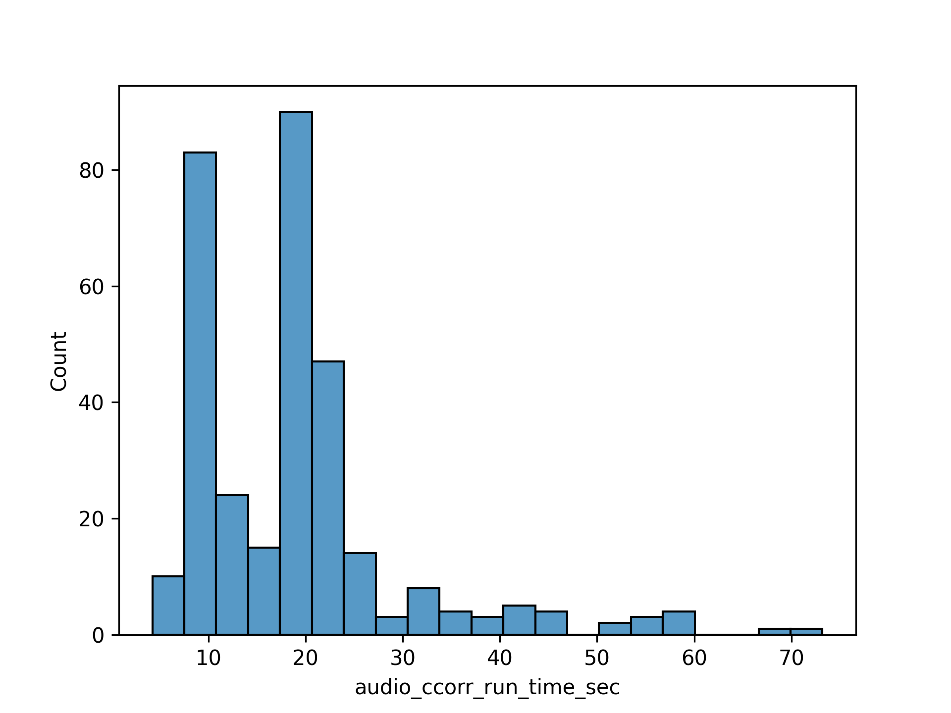Figure 1: Distribution of audio cross-correlation run times (in seconds) showing a bimodal distribution with peaks around 5-10 seconds and 20-25 seconds.

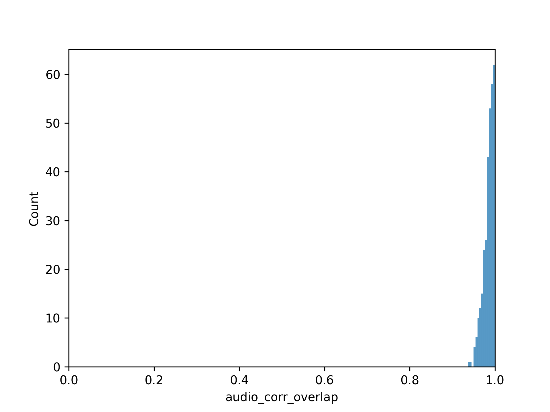Figure 2: Distribution of audio correlation overlap values, showing that most matches have overlap values very close to 1.0, indicating high accuracy.

Conclusions and next steps

When sound signals are unavailable, the audio-cross-correlation approach becomes useles. Instead one has to leverage the features of the image itself and its context. I have tested piecewise hashing, wavelet transform, and I am currently exploring more advanced embeddings to match the reliability of FFT. That will be the subject of a new article once I get the hang of it.

Code Base:

Feel free to clone: https://github.com/Haroldinho/audio_timestamp_extraction

References

1. Brunton, S. L., & Kutz, J. N. (2019). Data-Driven Science and Engineering: Machine Learning, Dynamical Systems, and Control (1st ed.). Cambridge University Press.
2. BBC. (2006). Planet Earth, Episode 1: From Pole to Pole. https://archive.org/details/planet_earth_1_bbc/planet_earth_01_from_pole_to_pole.mp4